INTERACTION BETWEEN DAYLIGHT AND WATER IN ARCHITECTURE THROUGH SIMULATION OF CAUSTICS
M. Di Sibio; O. Baverel
Ecole Nationale des Ponts ParisTech – Master Spécialisée Design by Data 2018-19
0 ABSTRACT
In the last decades, various computational approaches to the design field have started to emerge and become widely employed. Computational and generative design are, actually, mostly used in structural engineering, artistic installations, project management and performance-based design, while there are fewer examples of using those tools to study how certain phenomenon affect a building from a perceptive and architectonic point of view.
This study aims to provide a simple but robust framework to evaluate and study the interaction between daylight and water as a precise architectonic intention: the phenomenon of caustics will be studied and simulated. This framework is applied to a real case-study project currently developed by Ateliers Jean Nouvel, the intention of which is to understand the caustic effect in relation to the project, in order to enrich and inform the architectural design.
The problem of gathering useful and usable caustic data is addressed in this paper and an architectural design proposition will be done as an example of how to use the obtained data.
To validate the result, measurable images will be generated using both validated and proprietary rendering engines.
KEYWORDS: caustics, reflections, daylight, water, light, architecture
1 INTRODUCTION
In architecture, water and light, but more in general the relationship with nature, has always been very strong, and, in many cases, has been the tool used to guide the whole design process.
In architecture there are plenty of examples using light and water as physical architectural elements, like in the excellent work of Louis Kahn [11], Rem Koolhaas or Tadao Ando [12].
Therefore, it has been very difficult to find literature and works about the specific phenomenon of caustics in architecture, exception made for the work of Philippe Bompas (Fig. 1.1) [13].
Caustics are one of the most fascinating light phenomenon, consisting in the continuous focusing and diverging of light rays, creating refracted or reflected light patterns in a way that seems unpredictable, but once it takes place, curiously, shows lifelong stability and persistence [3]. Almost everything that can reflect or refract light can spot caustics: windows, glasses filled with liquids, metals or water (Fig. 1.2).
How can a random and wild phenomenon like caustics inform the architectural design process?The aim of this paper is to study caustics in order to find a simplified methodology to compute and predict this phenomenon and allow to use it as an architectural feature. It’s important to state that this research is not about controlling the shape or the pattern of reflected light, but instead to understand, when and where caustics will take place and define a convenient way of measuring this chaotic and apparently unpredictable effect. In a second section of the paper a simple algorithm will be developed in order to optimize the architecture geometry in relationship to the caustics.
Chapter 2 of the paper, will explain the background research made on caustics, give an overview of the actual studies on caustics and show some references of previous works on the subject.
Chapter 3 will state the objectives of this study and Chapter 4 will give an introduction to the case study and the design parameters.
In Chapter 5 the methodology proposed will be explained, as well as the models used, while Chapter 6 will explain the results obtained.
Chapter 7 will address the methods used to validate the methodology.
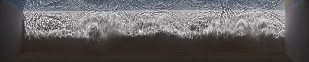
Fig. 1.1- Philippe Bompas, Lighwaves (2012); A fine layer of water refracting light passing through a transparent window.
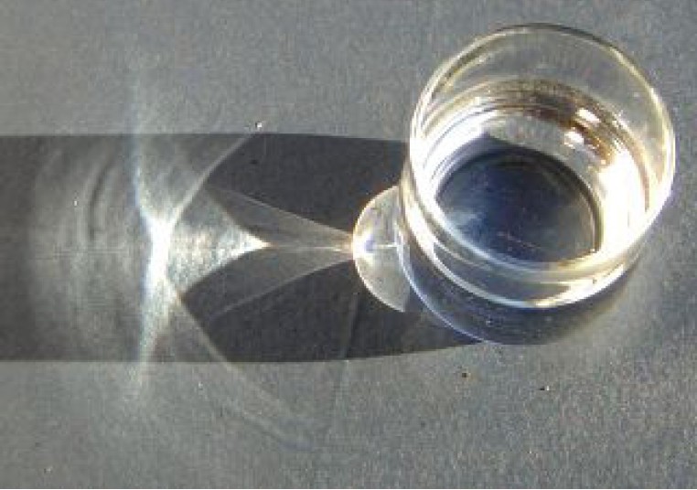
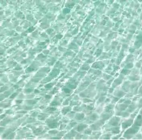
Fig. 1.2- A glass of water casting caustics (Left); Underwater caustics (Right)
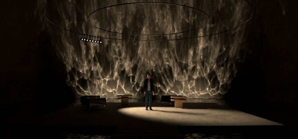
Fig. 1.3- A scene taken from the movie Blade Runner 2049 showing the work of Roger Deakins with caustics.
2 BACKGROUND RESEARCH
2.1 Caustics
When light propagates through a medium, especially a liquid in motion like water, is not occasional that it focuses and dim constantly in apparently random patterns. Those patterns are called caustics and, despite one can imagine, those are not just the focusing point of light travelling through a material acting like a lens, but in general are families of rays enveloping a caustic surface in space. This means that caustics are three dimensional structures of concentrated rays in space and that the simple focus point (of a parabola or sinusoid curve for instance) is still a caustic but is also unlikely to be found in nature due to its perfect symmetry and his high instability [0].
The term “caustic” comes from the ancient Greek word καυστός (kaustόs), that means “burnt” because of the nature of this phenomenon of concentrating rays and eventually, in specific cases, burn a surface [4].
Nowadays a caustic is not representing anymore a mystery but, before the end of the 70’s, the geometrical optics theory was not able to fully explain the phenomenon, until the introduction of the theory of catastrophes, which leaded to the creation of catastrophe optics theory. Today we know that a caustic basically represents a discontinuity point in a stable system (which is called a catastrophe) [0].
2.2. Related Works
Architecture literature is particularly rich regarding the theme of light and water. Those natural elements have been always seen as features to improve physical and psychological health of the human being, as highlighted also by several studies [15]. A special regard to light and water in architecture is due to the growing attention to sustainability, especially in the latest years, when computational power is enough to predict and optimize performance gains due to the combination of those elements.
Therefore, there is a lack of architectural studies on caustics. The work of Philippe Bompas on caustics is one of the closest to the actual architectural practice, in particular with Timescapes (Fig. 1.1), a project that investigates how light, water and other materials interacts each other. Another interesting work has been conducted by EPFL on the way a caustic can be controlled in order to produce an image, deforming a refractive surface of plexiglass [4].
Other examples of working with caustics can be found in cinema and photography, which are deeply correlated with the intention of this study of recreating a specific ambience for a non-controllable environment. Specifically, the work of Roger Deakis as light designer for some stages of Blade Runner 2049 has been very inspiring (Fig.1.3).
2.3 Metrics
In order to be able to express numerically such a raw and qualitative phenomenon, it is urgent to find a way to measure, somehow, the caustic effect. Based on the previous research (Chapt. 2.1), the fact that a caustic is a three-dimensional structure helps defining the main metric which will be the Thickness of the caustic surface, an indicator that can easily give a qualitative idea of the phenomenon as explained in Fig. 2.3.1. It is important to state here that the acceptable boundaries for this value are set empirically, based on experience and necessity, because of the aesthetic and unquantifiable nature of the problem. At the end of the workflow what is here called a Caustic Index will be produced in order to quantify in a scale from 1 to 0 the quality of the effect. Along with the Thickness, other metrics will be gathered and stored in order to be used and studied afterwards.
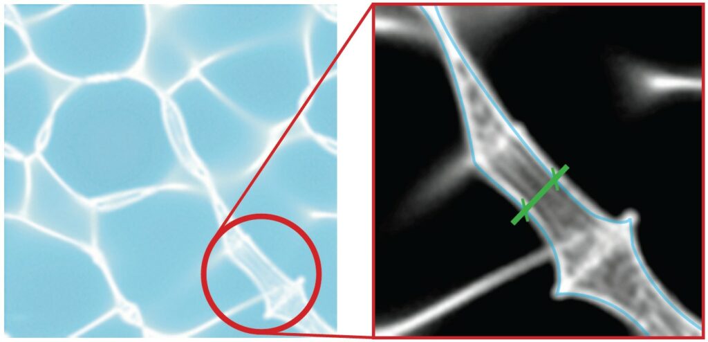
Fig. 2.3.1- (Left) Photography of an underwater caustic; (Right) A high
contrast zoom of the caustic showing in blue the bounds of the caustic
surface. In green is represented the measure corresponding to the average
Caustic Thickness metric.
3 OBJECTIVES
The aim of this study is to understand how caustics can become part of architectural design
process along with light and water. The outputs will be multiple and all related to the case study
currently developed at Ateliers Jean Nouvel: “heatmaps” and schemes showing during the
year and the analysis days the location, the characteristics and the Caustic Thickness metric (as
described in Chapter 2.3) useful to understand the overall behaviour of the caustics. Based on
that schemes and datas, placement of various architectural elements will be decided accordingly
in order to, locally, maximise or minimise the caustics.
Through the application to the case study, the main goal is to define a methodology to address
analytically the study of caustics, cutting the time for qualitative visualization (that actually is still
very high and often not enough accurate) and provide anyway consistent answers.
4 CASE STUDY
The case study is the Zhoushan Cultural Tourism Financial Complex (ZCTFC), a project actually
being developed at Atelier Jean Nouvel.
The site is located near Zhoushan, China, about 180Km south from Shanghai (Fig. 4.1) and is displaced
in two islands, it is obvious that the relationship with water is absolutely predominant.
The whole project consists in several interventions covering the entire surface of the two islands (Fig. 4.2), but for the purpose of this paper we will focus only on the building denominated Marine Horizons (Fig. 4.3), a terraced building that enhance the relationship between water and light as a main architectural feature; the concept, indeed, is inspired by the typical Chinese terraced rice fields.
The typical section of the building (Fig. 4.4) shows an intentional repetition of the same system (Fig. 4.4 top) for several floors and also suggests how strong will be the interaction of light and water, considered as an architectural feature but inevitably posing several problems that needs to be addressed. One of the most important desired effects of this interaction is represented by caustics, intended as a phenomenon aimed to improve the perceptive quality of the private terraces of the building; it is merely an aesthetic intention, but it represents a strong natural effect as well that is always been fascinating and can provoke positive psychological effects. The architectural features of the building we are most interested in, for this study, are represented by the apartments, the pools (1m deep), the water mirrors (0.15m deep) the and the overhanging terraces to serve as sunshades. Other important elements are represented by the ceiling windows that will be placed below the water mirror level, on the overhanging roof, and the pool vegetation that will serve for the Phyto depuration of the pool water. The roof windows, being below the water level, will cast refracted caustics in areas normally darker while the vegetation, placed above the water level, will help to block reflected light and for consequence reflected caustics in zone where this effect could be discomfortable causing glare and overheating, like in the interior of the apartments.
Those two elements are then interesting to be manipulated in order to control the caustics behaviour
during the analysis days. To summarize, among the others, one big intention of the project is to study how caustics can be implemented in the architectural design in order to significantly improve the ambiance and the quality of the space.
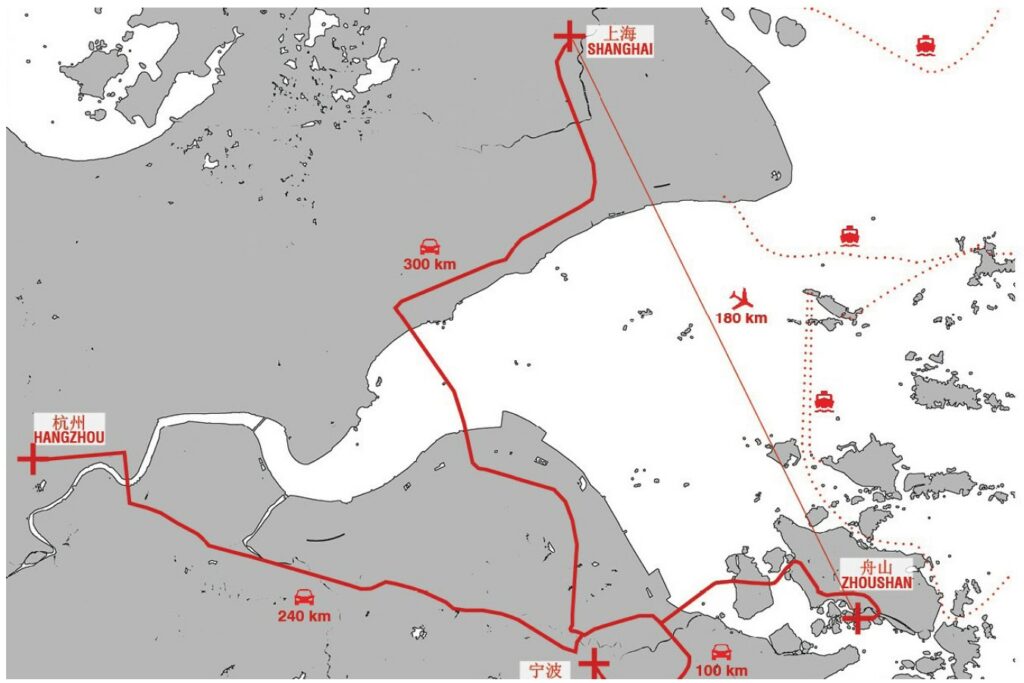
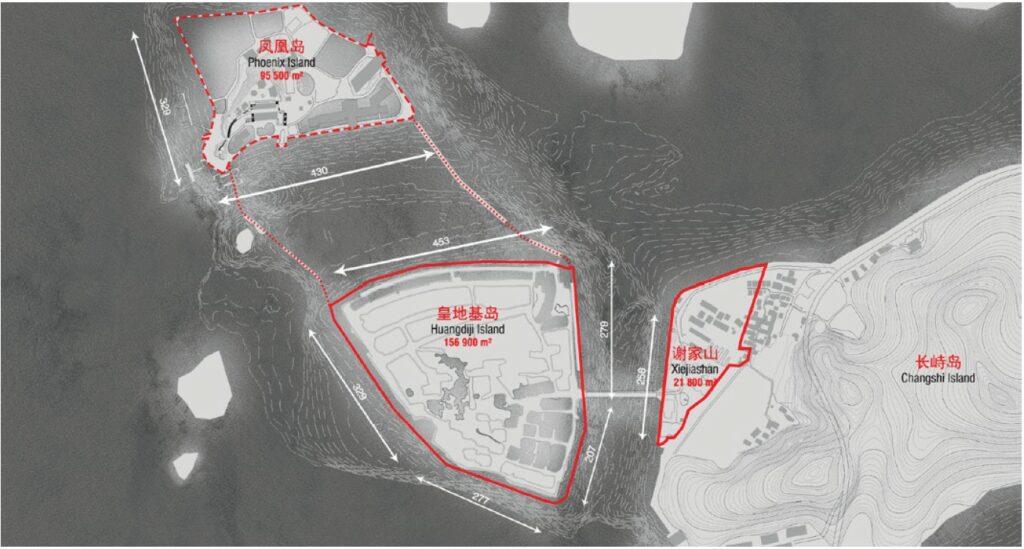
Fig. 4.1- Distance between Shanghai and Zhoushan
Fig. 4.2- Zhoushan; Site of the project
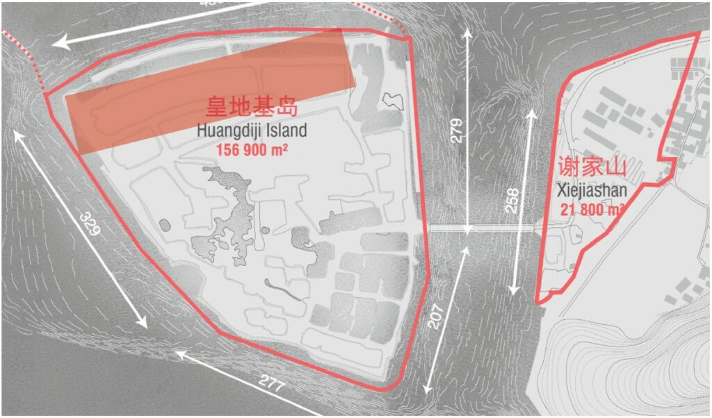
Fig. 4.3- Zhoushan; Marine Horizons location
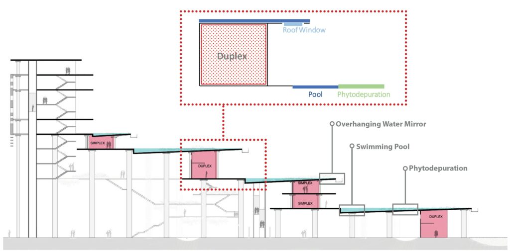
Fig. 4.4- Zhoushan Cultural Tourism Financial Center; Marine Horizons Typical Section of the building highlighting housing units (in red) and water pools (in blue). On top, a scheme of the elements composing the base system.
5 METHODOLOGY
In order to address the problem, the first step is evidently to understand how to properly simulate and measure the behaviour of caustics and gather necessary data.
At a first glance, one could think about using a classic photon mapping rendering engine in order to address the problem and visualise the results, but the drawbacks in this case are several: the very high computation time represents a huge bottleneck for the workflow, but the main problem is the lack of usable data. It is indeed hard and unprecise to analyse image data coming from rendering engines since in most cases is dominated by noise.
In this study is not relevant to visualize the caustic itself; it is relevant instead to have the possibility to rapidly calculate all the quantitative characteristics of a caustic for many different scenarios and situations in order to store them and reuse precalculated data afterwards. A methodology using geometrical optics theories is then proposed to solve a relatively small but still relevant amount of sun ray intersections and find the metrics described in Chapter 2.3.
5.1. General Workflow
The general workflow (Fig. 5.1) of this study can be divided in two standalone and linked models: an evaluation model will be used to pre-calculate and store generic caustics metrics for a broad range of sunlight directions and water wave conditions; on the other hand, the case study model is where gathered data will be used to calculate the actual conditions relatives to the case study and where statistics and metrics are analysed in order to retrieve the useful information. The two models will gather weather data from the Energy Plus online database of weather and sun conditions specifically for the Zhoushan area [16].
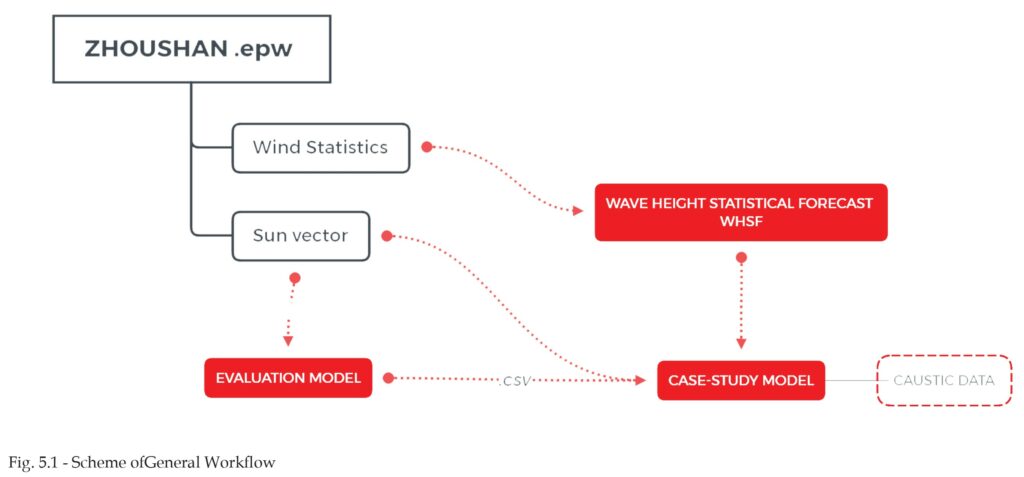
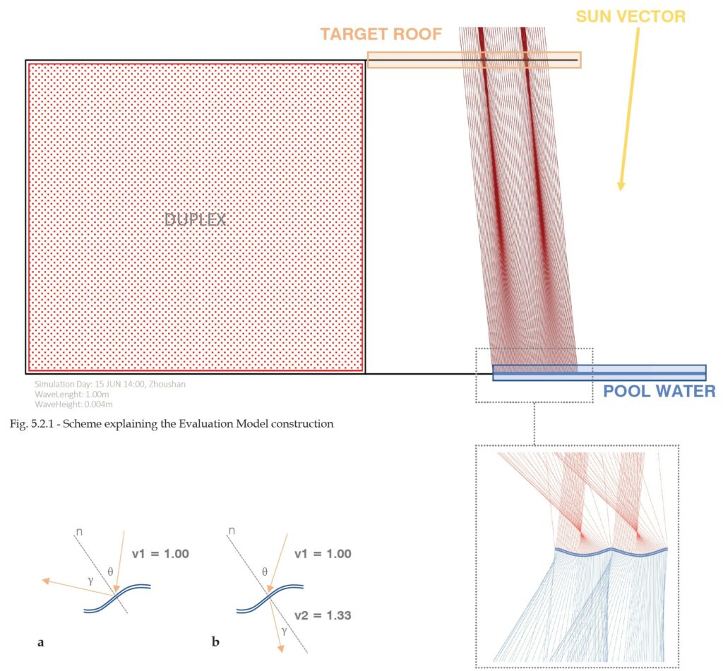
Fig. 5.2.2 – On the left (a) the calculation rules for reflected rays; on the
right (b) the scheme for calculating refracted rays. Both are using the
Snell’s Law.
Fig. 5.2.3 – Zoom showing the modeled trochoid wave curve (double blue
line), reflected rays (in red) and refracted rays(in blue)
5.2. Evaluation Model
The evaluation model is a parametric two-dimensional representation of the basic architectural system of the case study (Fig. 5.2.1), meant to pre-calculate the characteristics of caustics in every condition of light and wind in order to understand how those parameters are affecting the phenomenon on a yearly scale.
Both reflected and refracted caustics will be calculated using different metrics as output.
The model is composed by water, represented by a trochoid curve, a sun vector and a target plane (in this paper the target will be placed at 6.4m high relative to the water level). The parameters of the simulation are represented by the water wave height (ranging from 0.001m to 0.150m), the water wave period (from 0.01m to 1.00m, the sun direction vector (for 8760 hours in the location of the epw file) and the target plane height (6.4m).
As it could be seen from the workflow of the evaluation model (Fig. 5.2.4) the first step is to generate the water wave curve using the wave height and period parameters. For the purpose of this study, literature suggests [9] that the widely employed sinusoid curve is not the best suited for simulating water waves; it is instead the trochoid curve (or circular curve) (Fig. 5.2.3) the one that best approximates the shape and the motion of water with periodic waves, since in reality it is not a symmetric shape. The period of the curve, and of the model more in general, in this case, is needed in order to obtain consistent results between different tests. A random gaussian function could be used in place but this kind of curve will probably give false results due to the randomness.
Therefore, since the pools of this case study must be considered as shallow water, we assume that waves generated by wind (without external perturbations) in such conditions can be considered close to be periodic; the two wave parameters at this point are calculated using a brute force algorithm in order to retrieve every result. It is important to state that the model is computed using two periods of wave, in order to take into account, the interaction that could occur between near waves but keeping the algorithm very light, without sacrificing precision.
A simple mathematical raytracing script calculates then the interaction between a significant number of light rays (1000 in this case; 500 per wave period), also called samples, and the NURBS curve using the Snell’s Law (Fig. 5.2.2) [5] to determine the reflected and refracted angle of incidence:
sin θ/sin γ = v1/v2 {1}
where θ and γ are respectively the angles formed by rays with the normal to the wave and v1 and v2 are represents the density of the two different mediums.
Since the algorithm needs to calculate just one bounce of the rays, the calculation is very fast. The first families of rays are casted parallel to the sun direction vector and following the angle retrieved by the equation they determine the intersection point with the target plane.
A caustic is detected by the algorithm if at least the 5% of the total amount of rays intersects the target in the same spot or if their intersection forms a linear group of point which is smaller than the threshold T:
T = D(S-1) {2}
Where D is the average distance between the intersection points and S is the number of ray samples. Those values are determined experimentally, and various test shows that changing the number of rays does not affect significantly the results. the length of the group of intersections. The choice of using NURBS curves instead of using a traditional mesh is due to the necessity of extreme precision, hardly achievable with meshes since all the sample points are concentrated in two wave periods. The first attempts with traditional raytracing with high density meshes (edges smaller than 1mm) showed higher calculation time and a significant number of rays were falling in same face then wrongly calculated as parallel. The calculation is being done both for reflected and refracted caustics, gathering different metrics for each category. To give a further dimensional idea of the pattern that could be achieved in a particular condition, another gathered metric will be the distance between the centres of the neighbouring clusters, called Caustic Relative Distance. All these metrics are then stored along with their generating parameters in a .csv file in order to be reused afterwards. A slightly different and simpler process is used to gather the metrics for the refracted caustics. Since those are supposed to be casted from above, the most interesting data to analyse is how far from the media interface the caustics will start to be in focus (for example the distance between the water surface and the floor of a pool). To address this problem, the distance between the ground plane and the first intersection point is being calculated. The value will give an idea of the depth at which the caustic will start to be in focus and be appreciable. This value is then stored in the database. The process is repeated for each hour of the year (using Zhoushan, China, as location) and for each condition of water wave, using a brute force algorithm. It could be of course possible to already restrict at this point of the workflow the number of iterations, studying the weather and sunlight data of the site, but it is indeed interesting to visualise how different conditions are giving different result and the correlation between them. It is also a very fast process. More details are discussed in Chapter 6.1.
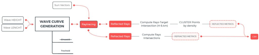
Fig. 5.2.4 – Evaluation model workflow
5.3. Case Study Model
The case study model represents the simplified architectural geometry of the Project of the ZCTFC and it has its own specific workflow (Fig. 5.3.2). An iteration floor-by-floor is necessary in order to reduce the computer memory usage and simplify the simulation; The algorithm gathers weather data from Energy Plus .epw file, a free online weather database that guarantees in general a good historical source of data [16]. In the case of this study, the data taken into account is the wind speed and direction, since they will inform the first part of the algorithm, the Wave Height Statistical Forecast [b6]. Literature describes this method as a way to forecast the wave height and period in open sea, but provides also a method to bound the results in order to be valid as well as for shallow waters. More details about this method will be explained in chapter 5.3.1. The WHSF will give as output the parameters of the wave, in order to retrieve the relative caustics data from the csv database previously generated with the evaluation model, along with the sun vector, calculated using Ladybug; those new metrics are stored in a second csv file for being analysed. In parallel, a daylight analysis made with Radiance will be performed using the ceiling of the terrace as target, in order to retrieve lit and dark zones. The process and the model are explained in Chapter 5.3.2. This data will be weighted with a Caustic Index (explained in chapter 5.3.3), to give an idea of where the effect will be maximum or minimum and at the same time to show different intensities of the phenomenon. The resulting map is what is called in the workflow scheme “Caustics Heatmap”. These maps will be used to design the vegetation areas needed for the pool Phyto depuration, in order to modify those heatmaps and maximise the quantity of caustic effect in allowed zone or block it in unwanted zones (like in the interiors of the apartments).
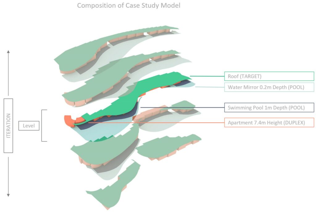
Fig. 5.3.1- Geometric composition of the case study. Highlighted a single floor.
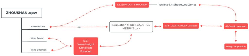
Fig 5.3.2 – Case Study Workflow
5.3.1 Wave Hight Statistical Forecast
An algorithm capable to estimate waves characteristics given the wind speed is the Wave Height Statistical Forecast (from here onwards called also WHSF) (Fig. 5.3.1.1) developed by US Army Corps of Engineers and described in the Coastal Engineering Manual [8]. In order to find the wave height limit Hmax, in relationship to the wind hourly data, the following equation needs to be resolved:
Hmax = (0.27U2) / g {3}
where U is the wind speed at the desired height and g is the gravity force.
To calculate U at a given height, the Wind Speed Calculator of Ladybug is used, in order to correct the .epw hourly wind data, which is calculated at 10m high.
The value obtained by {3} should be adjusted if it exceeds the values of the wave height Hw con-strained by the wind distance retrieved by the equation:
(gHw)/Uf2 = 4.1310-2 * ((gX)/Uf2)1/2 {4}
where Uf is the Friction Velocity if the Drag Coefficient is considered constant and X is the wind dis-tance, which expresses the distance in meters the wind can travel without physical obstacles.
Uf is calculated by the following expression:
Uf = Ux²(0.001(1.1+(0.035Ux))) {5}
Where Ux is the wind speed at 10m high.
The wave period maximum limit Tp is determined by the equation:
(gTp) / Uf = 0.751((g*X)/Uf2)1/3 {6}
This value, in case of shallow water, must be validated by performing the following actions:
- Check that Tp < Tmax; if Tp > Tmax, we assume Tp = Tmax;
Where Tmax = 9.78(d/g)^1/2 - Recalculate X using {6} for the corresponding boundary value and recalculate Hw using {4} ac-cordingly;
- If Hw > 0.6d then Hw = 0.6d
Where d is the water depth
The limits for using these formulas are primary regarding the wind speed, which must be below 37.5 m/s, above which the wind is considered a hurricane.
The distance X in the case study is largely sufficient to ensure that all the obtained values are never restricted by this parameter.
More limitations are explained by [8] and [10].
This algorithm returns the wave parameters Height and Period for each hour of the year, that will be used to retrieve the caustic characteristics.
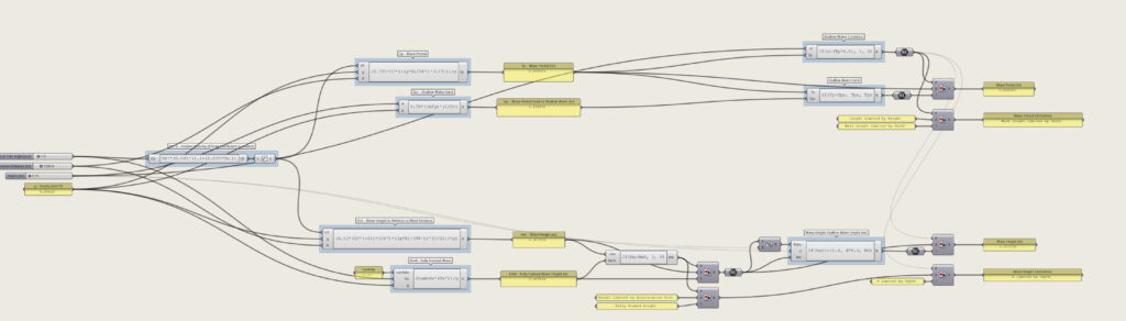
Fig.5.3.1.1 – Grasshopper Algorithm used to calculate WHSF
5.3.2 Daylight Simulation Setup
The daylight analysis is performed in order to retrieve for each floor’s target lit and dark zones.
The analysis is done using the Grasshopper plugins Honeybee and Ladybug, which allows to maintain a parametric workflow; the used engine is Radiance, a validated raytracing software capable of accurately simulate daylight.
The model is composed by several parts (Fig. 5.3.2.1a): the apartments are represented by their bounding boxes, the concrete terraces, the roof internal and external targets (Fig. 5.3.2.1b) and the pool water.
For each element is used the standard radiance material corresponding to the architectural functions (such as walls, floors, roofs, …) and for water a custom parametric material is used in order to account the Fresnel Laws, since the RGB reflectance of water changes according to the sun angle between its direction and the vertical vector Z [6].
To address the problem, the Schlick’s Approximation [7] of the Fresnel Equations is used; this formula is often used in computer graphics (Fig. 5.3.2.2):
R = R0+(1-R0)*(1-cos(θ))5 {7}
where θ is the angle between the direction of the sun and the normal to the interface of the two media and R0 is the reflection coefficient for rays parallel to the normal Z and R is the material reflectance.
R0 = ((v1-v2)/(v1+v2))2 {8}
Where v1 and v2 are the indices of refraction of the two media: in this case v1=1 (air) and v2=1.33 (water)
With this algorithm, the simulation takes into account the fact that in the morning and in the evening, water is reflecting more rays than at noon.
Since we need this analysis in order to understand where and when caustics happens, before the simulation the water surface is projected into the target roof following the sun direction vector inversed; the Boolean subtraction of the projection from the roof determine the zones in which, at the given sun conditions, is impossible to have caustics. (Fig.5.3.2.1c)
The analysis mesh resulting from Radiance (Fig. 5.3.2.1d) is then modified in order to set to a 0 Lux value all the sample points inside the found curve; the other values are remapped into a 0-1 value scale where 0 equals to 0 Lux and 1 equal to 100000 Lux (Fig. 5.3.2.1e).
The Radiance analysis is performed every 15 days of the year, for each hour from 9:00 to 16:00. A total of 168 analysis meshes are calculated along the whole year. Since in the global workflow we are working with hourly data, in order to be weighted with the Caustic Index, eight linear interpolations are done, one for each hour of the day, in order to obtain 2920 meshes; because night-time is not considered we don’t calculate the whole 8760 values.
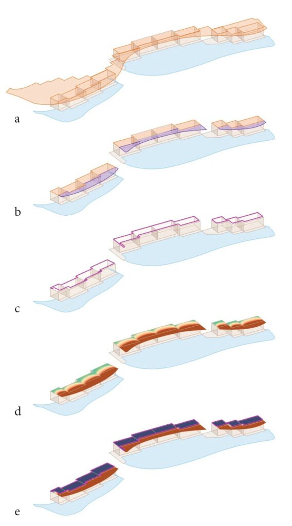
Fig. 5.3.2.1 – a. Radiance Model Elements; b. External Target in purple
and Internal Target in orange; c. Area in which caustics are not possible;
d. Radiance analysis mesh: e. Radiance analysis mesh corrected and
remapped.
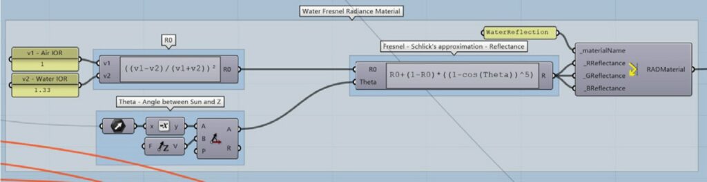
Fig. 5.3.2.2 – Grasshopper Algorithm used to calculate Schlicks Approximation
and Radiance Mirror Material used for Water
5.3.3 Caustic Index
As stated before, the aim of this research is mainly to understand how to express numerically a chaotic and qualitative effect such as caustics. In a first step some characteristics such as thickness and relative distance are calculated, but in order to evaluate the caustic quality globally, an index ranging from 0 to 1 is needed and easier to use.
With all the gathered data from the precalculated database, we can rapidly build a second database relative to the case study, this time recording the caustics for each hour of the year in Zhoushan using real wind and sun data to extract the metrics.
This last database shows that, excluding the +Infinity values, which means the caustic is out of focus, the boundaries of caustic thickness in this geographical area are ranging from 0.001m to 0.52m.
The first operation done is to replace every infinite value with the upper bound 0.52m and remap those values into 0-1 domain.
The following formula is then applied:
abs|CT-CTd|-1 {9}
Where CT is the Caustic Thickness and CTd is the Desired Caustic Thickness (Target Value);
The CTd value used is 0.05, since in this case the most desirable caustic thickness is 5cm; the {9} equation makes an offset of every value in order to set 5cm at the 0. The -1 exponent is needed in order to reverse the domain: the result is that 1 will correspond to 5cm and 0 will correspond to 52cm thickness.
This index is used afterwards to be multiplied with the luminance 1-0 value in order to retrieve the results.
The output is a dataset of 8760 values, ranging from 0 to 1, which are representing the Caustic Thickness for each hour of the year.
6. RESULTS
This chapter will discuss about the obtained results both for the evaluation model and the case study model.
6.1. Evaluation Model
The results obtained from the caustic evaluation model are formatted in a csv file containing all the combinations of Wave Height, Period and sun direction for each hour of the year in Zhoushan.
The 15 July at 14:00 dataset resulting from the evaluation model is then visualized (Fig. 6.1.1) in order to make the gathered data easily readable. The metric visualized by color gradient is the Caustics Thickness, which has been culled to a maximum value of 20cm, empirically. It is noticeable how actually is the wavelenght the parameter that most affects the results, except for very short waveheights. It is also interesting to see how the Caustic Thickness tends to grow while the wavelenght grows, but at certain point it starts to decrease again; this phenomenon is caused by the interference between two near waves.
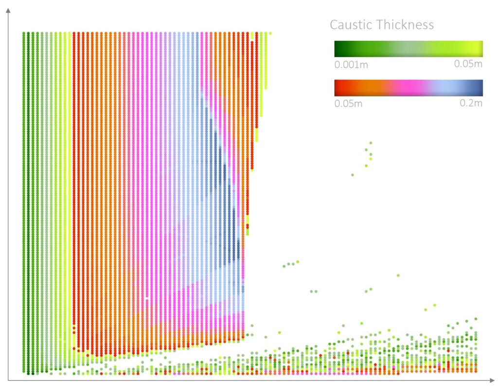
Fig. 6.1.1 – Evaluation model results visualization. X axis – wavelenght (0.01m – 1.00m); Y axis – waveheight (0.001m – 0.15m). Colours are representing the Caustic Thickness calculated at 7.4m high (ref legend on top).
6.2. Case Study Model
The first operation done in order to retrieve the first results is to weight the luminance values of each Radiance mesh with the Caustic Index.
The mesh values are linearly interpolated and, taken alone does, not represents interesting results; on the other hand the Caustic Index is calculated for each hour; it makes sense then to weight every mesh with the corresponding Caustic Index, since are both ranging from 1 to 0 and since we want to weight caustic data with light brightness data.
We obtain 2920 weighted meshes with values ranging from 0 to 1 which represents the zones in which caustics are brighter or darker taking into account their thickness. From this data we can extract the average caustic per year (Fig. 6.2.1), the day of maximum and minimum values and it’s possible to visualize the heatmaps day by day.
In Fig. 6.2.1 it’s shown one floor (entire result in Fig 6.2.4) of the resulting mesh after making the average between all the obtained meshes for the whole year: it’s clear how the resulting colours are segmented in defined zones; the blue areas shows that generally at the bottom of the apartments will never happens caustics during the year; on the other hand the exterior overhang presents several areas in which on average caustics will takes place during the year. It’s remarkable to see how in general caustics are more concentrated on the east and west sides of the roofs, probabily because are casted in the late afternoon or in the early morining (Fig6.2.7 for comparison between caustic wind and su altitude). It is interesting also to see how at level F1 (Fig. 6.2.4) the middle roof is the one that presents more caustics overall: it can be explained by the half floor-to-floor height of this level and, since there are no pools below this portion, another time those are caused by early morning or evening rays. This result shows how the important height between levels is making caustics more difficult to percieve.
Analysing the data presented in Fig. 6.2.5 shows that the day with the best caustic conditions is 30 July at 16:00 and the un position can be seen in Fig. 6.2.4; the wind speed is relatively low at 4m/s (7.78 Knots) but enough to produce some small waves.
On the other hand, the worst day is September the 14 at 10:00 with wind speed of 12 m/s (23 Knots) which is very close the upper bound of the wind dataset (Fig. 6.2.6). It is important to note that the site during the year is not very windy, and the upper registered bound is 14.9 m/s registered the 20th September at 20:00.
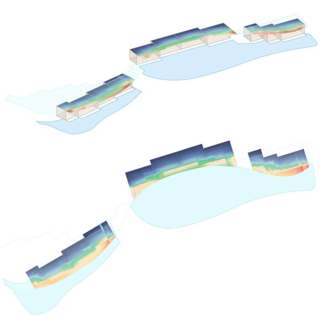
Fig. 6.2.1 – (Top) Axonometry of the case study’s first floor model showing the average of all year’s days. (Bottom) Plan view; Colour scale used is the same as Fig. 6.2.1
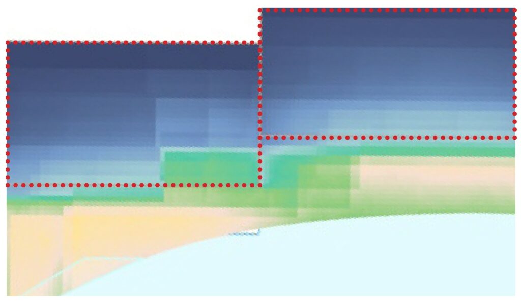
Fig. 6.2.2 – Detail Plan View showing the sharp edges caused by the average. Color scale used is the same as Fig. 6.2.1; The red dotted line represents the apartments bounding box.
7. VALIDATION
This chapter presents the methodologies used in order to check and validate the accuracy of the proposed workflow for the Evaluation Model.
The validation process consists in the visual assessment of the results obtained by the algorithm and a second check using validated software Radiance.
The software utilized for visualization is Octane Render’s PMC Kernel, a rendering engine specifically studied for rendering caustics [14].
This engine can calculate extremely accurate caustics.
In the case studied, periodic waves are used in order to be able to measure effectively the numerical results: the caustic thickness and the relative distance between the clusters of rays.
After the calculation of the 8760 caustics metrics for each hour of the year in Zhoushan, using the WSHF algorithm for determining the wave conditions, 15 March at 12:00 is chosen as validation day since is the closest to a 10cm thickness caustic (0.09989m), which is convenient to measure. Furthermore, the caustic relative distance is 0.299m which is also very handy to measure.
The calculated wave period is 0.29m and the wave height is 0.003m. (Fig 7.1)
The wind speed at 7.4m high, which is the lowest pool in the project, calculated using Ladybug Wind Speed Calculator component for Grasshopper, is 0.774 m/s.
The Radiance analysis (Fig.7.3 Top), performed on the sample portion of the project, clearly shows horizontal high contrast zones with a difference of more than 15000 Lux. Using a 5x5cm mesh grid as analysis surface permits to appreciate the phenomenon, since the caustic should be the double in dimension (10cm) (Fig 7.3 Bottom). The high contrast zones are affecting 2 consecutive faces and are on average distant 30cm each other. The results are then coherent with the evaluation model.
For the visualization assessment, Octane PMC Kernel is used to render the same model used for the Radiance Analysis, in order to visually confirm the results (Fig 7.2 Top).
Exactly the same zone and time is used and, as precaution, every image filtering, post production colour correction or denoising feature is turned off. A parameter intended to speed up the visualization of caustics using interpolation, called “Caustic Blur”, is reduced to 0, which introduces artifacts and noise in the final image but gives unfiltered results.
At the 9x18m target roof surface is applied a metric checkerboard texture representing 50x50cm squares, in order to visually understand the proportions.
Fig 7.2 (Bottom), is a parallel view of the roof target seen from below, showing clearly the 10cm caustics with a 30cm space between them.
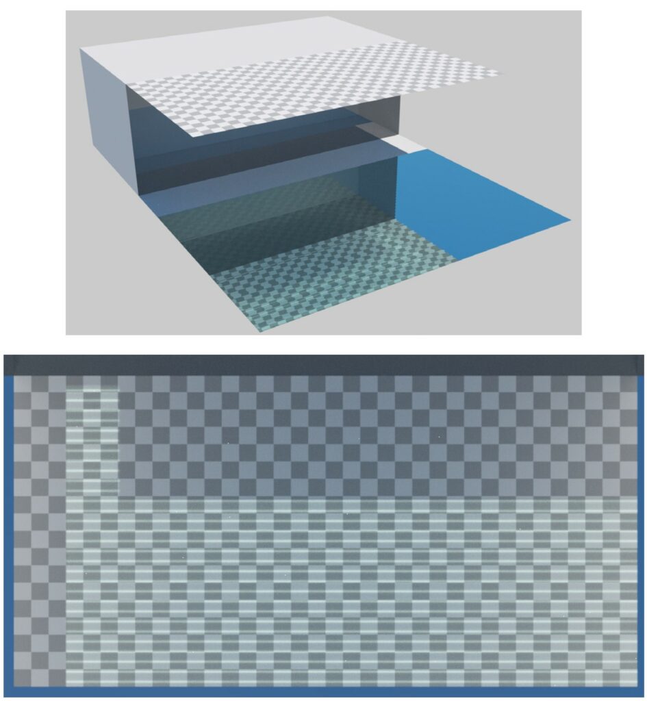
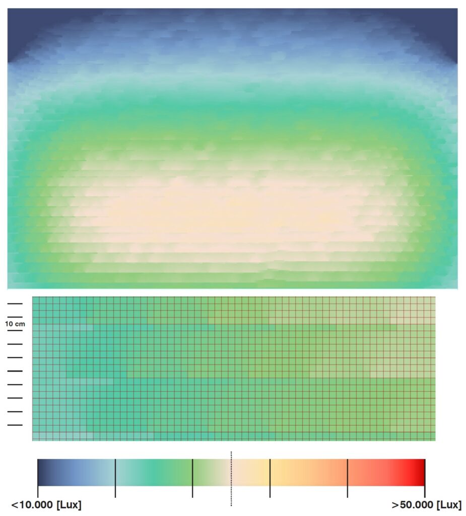
Fig.7.2 – (Top) Render of the 3D evaluation model with Octane PMC. (Bottom) Rendered bottom view of the target roof (18x9m); Caustics are visible over a metric texture. Each square has 0.5m side.
Fig. 7.3 – (Top) Radiance analysis plan view. (Bottom) Detail of the result mesh; Each face is 0.05×0.05m.
8. CONCLUSIONS
Despite the complexity of the phenomenon, it is interesting to see how, using a relatively simple algorithm, it is possible to understand how caustics are behaving in different conditions, by greatly simplifying the problem. Furthermore, it is interesting to see the different conditions in which caustics can happens during the year, and to discover that basically those are casted during the whole year but mainly in months where the sun is on average lower on the horizon and the wind conditions are not at the extremes.
On the other hand, it is very difficult to forecast caustics in standardized conditions, because of the huge number of parameters combinations that can produce caustics and that are not easily predictable.
9. ACKNOWLEDGEMENTS
The author wishes to thank Oliver Baverel, Adrien Rigobello, Romain Mesnil, Francesco Cingolani and Andrea Graziano for the precious help, advice and comments, a very special thanks to Tristan Israel for his support and dedication. Finally, a big thanks to all the students of the Master Specialisée Design By Data 2018-19 for their support and comments.
10. SOFTWARES
This research and all the described algorithms have been mainly developed using the 3d modeling softwares Rhinoceros and the plugin Grasshopper to develop the parametric workflow.
All the daylight analysis, both for the simulations and the validation, are conducted using Radiance as part of the Ladybug and Honeybee plugins for Grasshopper.
The last software is Octane Render 4.1, used for the visual validation since is among the most advanced physiscally-based engines capable of rendering caustics using GPU calculation and hugely reducing calculation time.
9. REFERENCES
CAUSTICS AND OPTICS
[0] CATASTROPHE OPTICS: MORPHOLOGIES OF CAUSTICS AND THEIR DIFFRACTION PATTERN; M.V.Berry, C. Upstill; H. H. Wills Physics Laboratories, University of Bristol. 1980
[1] CAUSTICS AND SYMMETRIES IN OPTICAL IMAGING. THE EXAMPLE OF CONVECTIVE FLOW VISUALIZATION; A. Joets, R. Ribotta; Laboratoire de Physique des Solides, Université de Paris Sud; 1994
[2] USING ROLLING CIRCLES TO GENERATE CAUSTIC ENVELOPES RESULTING FROM REFLECTED LIGHT; Jeffrey A. Boyle; Department of Mathematics, University of Wisconsin-La Crosse.
[3] NATURE’S OPTICS AND OUR UNDERSTANDING OF LIGHT; M.V.Berry; H. H. Wills Physics Laboratories, University of Bristol; 2014
[4] ARCHITECTURAL CAUSTICS: CONTROLLING LIGHT WITH GEOMETRY; T. Kiser, M. Eigensatz, M. Nguyen, P. Bompas, and M. Pauly; Advances in Architectural Geometry, Springer; 2012.
[5] FONDAMENTI DI FISICA; D. Halliday, R.Resnick, J.Walker; Zanichelli; 2001
[6] https://en.wikipedia.org/wiki/Fresnel_equations
[7] AN INEXPENSIVE BRDF MODEL FOR PHYSICALLY-BASED RENDERING; C. Schlick; Computer Graphics Forum; 1994
WATER, WAVES AND WIND
[8] COASTAL ENGINEERING MANUAL; U.S. Army corps of engineers; 2008; Chapter II-2-2, Pag II-2-37
[9] http://hyperphysics.phy-astr.gsu.edu/hbase/Waves/watwav2.html ; R.Nave; Georgia State Univeristy
[10] https://planetcalc.com/4442/
ARCHITECTURE
[11] BETWEEN SILENCE AND LIGHT: SPIRIT IN THE ARCHITECTURE. SHAMBHALA; L. Kahn; 1979
[12] LIGHT REVEALING ARCHITECTURE; Marietta S. Millet; Wiley; 1996
[13] https://philippebompas.com/
OTHERS
[14] https://docs.otoy.com/StandaloneH_STA/StandaloneManual.htm#StandaloneSTA/PMCKernel.htm ; Octane’s Render PMC Kernel Documentation
[15] https://www.archlighting.com/technology/the-benefits-of-natural-light_o ; « The Benefits of Natural Light »; Kevin Van Den Wymelenberg.
[16] https://energyplus.net/weather-location/asia_wmo_region_2/CHN//CHN_Zhejiang.Dinghai.584770_CSWD